Logistic Regression
Sigmoid
Logistic regression lesson goes immediately after Linear Regression, and instead of usage
predicting scalar number it is used for binary classification and predicts the probability
of an observation belonging to a particular class. It models the relationship
between input features (parameters) and the binary outcome (0 or 1).
The output of logistic regression is transformed using the logistic function
(sigmoid), which maps any real-valued number to a value between 0 and 1. This
transformed value can be interpreted as the probability of the observation
belonging to the positive class.
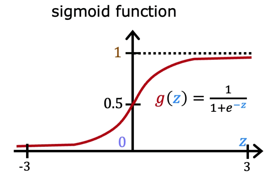
Logistic function is also known as sigmoid function. It compressed the output of
the linear regression between 0 and 1. It can be defined as:
\( z = \theta^T \cdot X \)
\( S(z) = \frac{1}{1 + e^{-z}} \)
Where z is output of linear regression, theta are learnable parameters and X is feature vector of you inputs.
It basically means than smaller output of linear regression is then smaller probability class 0 and vice versa with class 1.
Picture below demonstrates this effect.

Sigmoid function is accurately separating the classes for binary classification tasks. Also, it produces continuous values exclusively within the 0 to 1 range, which can be employed for predictive purposes.
This function will be used in future to understand how Some Reinforcement Learning Algorithm for example works.
We will learn parameters theta that allows our Agent Achieve the highest possible Reward in Environment.
We will manually calculate derivatives of this Model/Policy that allows transparently understand how works one of Base RL
and my favorite Algorithms REINFORCE, and after it will help us smoothly switch this model inside algorithm into more complicated models for example
Neuron Networks which we will be learning soon in a few lesson ahead.
In future we will need not only sigmoid function but also it's derivative. This function is useful and becomes in handy
for example as last layer of Neuron Network. As last layer for forward pass we use it and
it's derivative is used for gradient calculation of backward pass.
So i decided to pin its graphic here as already now.
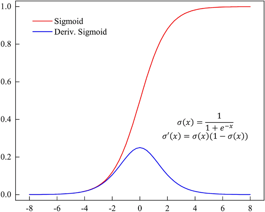

As small home task you can calculate its derivative manually using chain rule and other calculus rules to obtain same formulas
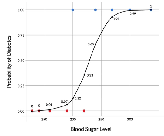
Example of usage logistic regression is presented below. You can use it for purpose
wheather person has or doesn't have diabetic disease based on sugar level in his blood.
Then more sugar you have then higher probability and tries to figure out what is the most
accurate separation line of these two classes.

What is Cost Function?
A cost function is a mathematical function that calculates the difference
between the target actual values (ground truth) and the values predicted by the
model. A function that assesses a machine learning model’s performance also
referred to as a loss function or objective function. Usually, the objective of a
machine learning algorithm is to reduce the error or output of cost function.
As you remember in Linear Regression the conventional Cost Function is the Mean
Squared Error. Formula below for one sample
\( \text{Cost} (\hat{y}_i, y_i) = \frac{1}{2} (\hat{y}_i - y_i)^2 \)
The cost function J for m training samples can be written as:
\( \text{J(θ)} = \frac{1}{m} \sum_{i=1}^{m} \text{Cost} (\hat{y}_i, y_i) = \frac{1}{2m} \sum_{i=1}^{m} (\hat{y}_i - y_i)^2 \)
but it is not suitable for logistic regression due to its nonlinearity introduced by the sigmoid function.
In logistic regression, if we substitute the sigmoid function into the above MSE
equation, we get:
\( \text{J(θ)} = \frac{1}{2m} \sum_{i=1}^{m} (\frac{1}{1 + e^{-(\theta^T \cdot X )}}- y_i)^2 = \)
\( \frac{1}{2m} \sum_{i=1}^{m} (\frac{1}{1 + e^{-(\theta_1 \cdot X_i + \theta_2)}}- y_i)^2
\)
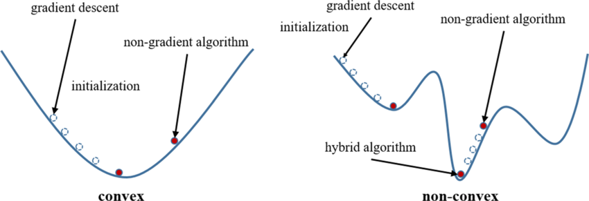
This equation is a nonlinear transformation, and evaluating this term within the
Mean Squared Error formula results in a non-convex cost function. A non-convex
function, have multiple local minima which can make it difficult to optimize using
traditional gradient descent algorithms as shown below.

We should find another cost function instead, one which has the same behavior
but is easier to find its minimum point.
Let's plot the desirable cost function for our model.
Our actual value is y which equals 0 or 1, and our model tries to estimate
it as we want to find a simple cost function for our model.
For a moment assume that our desired value for y is 1. This means our model is
best if it estimates y equals 1. In this case, we need a cost function that
returns 0 if the outcome of our model is 1, which is the same as the actual
label. And the cost should keep increasing as the outcome of our model gets
farther from 1. And cost should be very large if the outcome of our model is
close to 0.
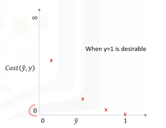

Model \( \hat{y} \)
Actual Y value equal 0 or 1
if Y = 1, and \( \hat{y} \) = 1 -> cost = 0
if Y = 0, and \( \hat{y} \) = 1 -> cost = large
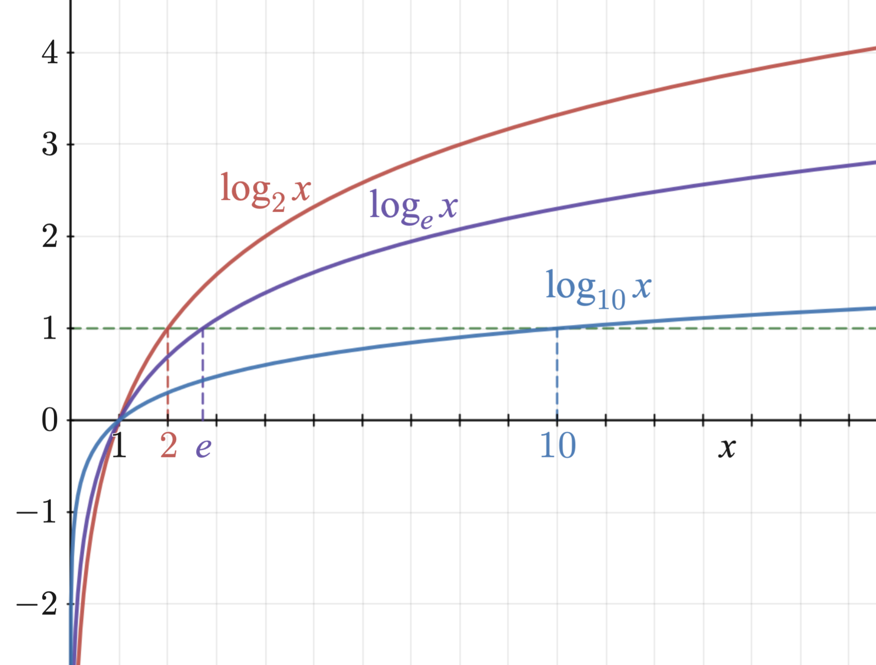
Let's repeat logarithm function and its behaviour. We are mostly interested in range [0,1].
if you multiply this function to -1 it will be very similar and good approximation of function
points examples on the picture above.

We can see that the minus log function provides such a cost function for us.
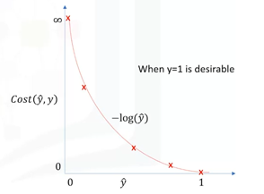

It means if the actual value is one and the model also predicts one, the minus
log function returns zero cost. But if the prediction is smaller than one, the
minus log function returns a larger cost value. So, we can use the minus log
function for calculating the cost of our logistic regression model. So, if you
recall, we previously noted that in general it is difficult to calculate the
derivative of the cost function. Well, we can now change it with the minus log of
our model. We can easily prove that in the case that desirable y is one, the cost
can be calculated as minus log y hat, and in the case that desirable y is zero
the cost can be calculated as minus log one minus y hat. Now, we can plug it into
our total cost function and rewrite it as this function.
\[
\text{Cost} (\hat{y}_i, y_i) =
\begin{cases}
-log(\hat{y}) & \text{if y = 1} \\
-log(1-\hat{y}) & \text{if y = 0}
\end{cases}
\]
\( \text{J(θ)} = \frac{1}{2m} \sum_{i=1}^{m} (y_i * -log(\hat{y_i}) + (1-y_i) * -log(1-\hat{y_i})) \)
Here you can notice that our loss function consists of two parts. Our values/labels are 0 or 1.
One of loss elements becomes zero and we work exactly with loss of class our label.
So, this is the logistic regression cost function which is called Log Loss
or Cross Entropy function. As you can see for yourself it penalizes
situations in which the class is zero and the model output is one, and vice versa.
- Case 1: If y = 1, the true label of the class is 1. Cost = 0 if the predicted value of the y is 1 as well. But as predicted value of y deviates from 1 and approaches 0 cost function increases exponentially and tends to infinity
- Case 2: If y = 0, that is the true label of the class is 0. Cost = 0 if the predicted value of the y is 0 as well. But as predicted value of the y deviates from 0 and approaches 1 cost function increases exponentially and tends to infinity which can be appreciated from the below graph as well.
Remember, however, that Model output y does not return a class as output, but
it's a value of zero or one which should be assumed as a probability.
Now, we can easily use this function to find the parameters of our model in such
a way as to minimize the cost.
Now we can use gradient descent to find optimal parameters. Approach is identical
we considered in the previous part for linear regression.
What is gradient descent?
Generally, gradient descent is an iterative approach to finding the minimum of a
function.
Specifically in our case gradient descent is a technique to use the derivative of
a cost function to change the parameter values to minimize the cost or error.
How can gradient descent do that?
Think of the parameters or weights in our model to be in a two-dimensional space.
For example, θ1, θ2 for two feature sets.
We need to minimize the cost function J which is a function of variables θ1 and θ2.
So, let's add a dimension for the observed cost, or error, J function.
Let's assume that if we plot the cost function based on all possible values of θ1, θ2
Multinomial logistic regression
This approach is a classification method that generalizes logistic regression
to multiclass problems, i.e. with more than two possible discrete outcomes.
We use the softmax function or normalized exponential function converts a vector
of K real numbers into a probability distribution of K possible outcomes.
\[
\text{Softmax}(x_i) = \frac{e^{x_i}}{\displaystyle\sum_{j=1}^{n} e^{x_j}}
\]
S;/.oftmax applies the standard exponential function to each element zi of the input
vector z (consisting of real numbers), and normalizes these values by dividing by
the sum of all these exponentials. The normalization ensures that the sum of the
components of the output vector ϭ(z) is 1.
The multinomial logistic loss is actually the same as cross entropy.
\[
\text{Log Loss} = -\frac{1}{m} \sum_{i=1}^{m} \sum_{k=1}^{K} y_{ik} \log(p_{ik})
\]
where m is the sample number, K is the class number.
\[
\text{Log Loss} = -\frac{1}{N} \sum_{i=1}^{N} \sum_{k=1}^{K} y_{ik} \log(p_{ik})
\]
That is it now for Log regression. This will be used in future as everything we learn here.