Why do we start with linear regression? Because it’s beautiful, first of all.
It’s easy to explain important basics of Machine Learning and the concepts of
deep learning with the following example. We will need deep learning, because modern RL
stands on this foundation.
Things you must understand after reading:
1) What derivatives and gradients are and why we need them;
2) The regression problem, how linear regression is built, metrics for linear
regression, peculiarities, and different special cases, and why the aforementioned
things happen the way they do;
3) How Stochastic Gradient Descent (SGD) works and the details of its implementation
from scratch. We will be using pure Python.
Part 1. Derivatives and gradients
The definition of the derivative is as follows, and this is where it comes from.
We remember two definitions of derivatives: physical and geometrical.
The definition below is geometrical.
The derivative of the function \( f(x) \) with respect to \( x \) is defined as:
So, what does it really mean? We remember that the gradient shows how fast the function
changes. The derivative is a function! The gradient is a scalar number – a concrete
number of this function at a defined point x, which shows how fast the function grows
or decreases at this precise point. When there’s a positive gradient number, the
function increases; but when there’s a negative gradient number, the function decreases.
When the gradient equals 0, the function neither grows nor declines. These rules hold
true as Δx tends to 0.
The formula for the derivative comes from the graph below. You should look at it and
match the formula with the graph.
Then, the faster and steeper the function changes at that particular point,
the larger the ratio proportion (numerator to denominator) will be, hence the gradient.
Also, we have noticed the second thing: if the gradient is a positive number
\( f(x + \Delta x) - f(x)>0 \), then the function grows (when we take a small
step to the right). Otherwise, \( f(x + \Delta x) - f(x)<0 \) and the function
decreases; the numerator of the fraction is a negative number, hence the gradient
is negative.
Then, the higher the absolute value of this number \( f(x + \Delta x) - f(x)>0 \)
(value in the picture above), the greater the gradient. This means that the function \( f(x + \Delta x)\)
at the point \( x + \Delta x \) differs significantly from the value at point \( x \)
. If the difference is significant, it indicates rapid growth or decline.
We can determine whether the function is increasing or decreasing by the sign of the
gradient. If the gradient is positive, the function is increasing. Otherwise, it is
decreasing or remains unchanged.
A) \( f(x + \Delta x) - f(x)>0 \) function grows;
B) \( f(x + \Delta x) - f(x)<0 \) function decreases;
C) \( f(x + \Delta x) - f(x)=0 \) remains the same.
Back in school, we were taught that the gradient of a line equals the tangent of
the angle of inclination alpha. This explanation directly relates to the definition
shown in the picture above, concerning the right triangle.
On pictures:
a) \( a>0 \) picture a - line grows;
b) \( a<0 \) - line decreases;
c) \( a=0 \) - it’s parallel x and stays the same.
Example with some numbers is below.
The main thing to remember about gradients is that they show us how a function changes:
how fast it changes and whether it grows or not.
This concludes the section on gradients and derivatives.
Now, let's apply our knowledge of gradient properties to a concrete example.
The task of linear regression is to construct a line that best approximates
points with the smallest error.
Gradients can help us to adjust the line's parameters to minimize this error and thereby better
approximate the points. We can calculate gradients for any differentiable function.
The SGD algorithm aids us in minimizing the Mean Squared Error using these gradients.
We can achieve this by leveraging gradient properties to update parameters. Gradients
indicate whether the error will increase or decrease if we adjust a specific parameter
of the line. We can apply this process to all parameters. Ultimately, our goal is to
reduce the error, so we adjust all parameters in the direction opposite to the gradients.
After n iterations, we check for any stopping conditions and halt the SGD algorithm.
Now we are ready to build Linear Regression. We can formulate our task as follows:
Firstly, mathematically: we have a set of points (possibly thousands) and we want
to approximate them with a function that best fits our data (minimizing error).
This is crucial because once we have this rule, we can predict values for other
points where the answers are unknown. The first step is to determine which type of
approximation function to use: linear, non-linear, polynomial, quadratic, trigonometric,
etc. Different datasets exhibit different patterns. To better understand this concept,
consider the example of the Anscomba dataset, which illustrates examples when use it or not.
You can load this dataset for example from seaborn package
These 9 points in each graphic share the same statistics such as mean and standard
deviation, but their representation and patterns differ significantly.
The top-left graphic exhibits a linear pattern, making it a suitable candidate for
Linear Regression;
The top-right graphic displays a quadratic pattern, best approximated by a parabolic function;
The bottom-left graphic includes an outlier. It's crucial to remove outliers and
correlated features before applying machine learning algorithms, as they can
significantly impact the final result;
The bottom-right example also does not fit well with a linear function application.
Ultimately, the choice of function for point approximation depends on your specific task,
its physical implications, and your desired outcomes.
Keep this mem in mind.
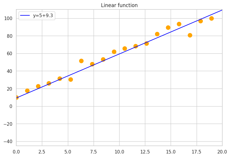
Let’s consider a training dataset, illustrated by the orange points in the graphic
below. Each orange point can be represented as (x, y), where x is a feature and y
is a scalar target or outcome. In more complex scenarios, x may not be a single value
but a vector of values, where each value describes a different attribute of an object.
Our goal is to find a line that minimizes the error, such as the Mean Squared Error
(MSE), which measures the average squared distance of all points from the line.
Another way to frame this task is as follows: Imagine explaining this problem to
children. Picture a scenario where all the orange points represent citizens in a large
city or village. Suppose there is no nearby river, but it's essential to dig a canal to
provide water for daily needs. Through a voting process, we need to decide where and
how to dig the canal so that all citizens are generally satisfied, and the overall
satisfaction of the entire village is maximized. How do we measure the satisfaction
of each citizen? By their distance to the river (represented by the blue line in the
graphic). The greater the distance, the less satisfied the citizen. In our context,
we use the square of the distance (since the derivative of a quadratic function is
linear, making gradient calculation computationally straightforward). We need to
determine the optimal locations to dig these canals for any number of citizens (points)
and their specific locations (x and y coordinates). Similar problems can arise
frequently. Additionally, if new citizens join the city or village, we should be
prepared to adjust our canal plans accordingly.
The important thing to mention that we can get the parameters for line equation using
statistics without SGD, but for our study purposes we will use SGD, because we will use
this SGD optimizer, as well as other in our RL projects many times, so we have to know
the way it works. This is one of the purposes this linear regression article.
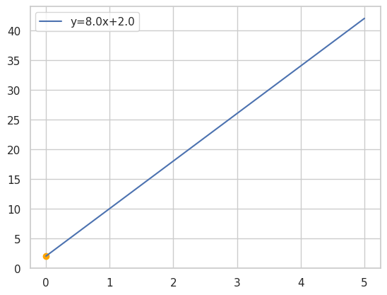
Let’s assume the initial proposal for the canal’s path is depicted below. The orange
points represent citizens, and the blue line indicates the proposed canal location.
Proposed canal location and citizens
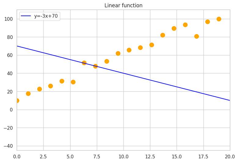
If we start with this initial suggestion, all the citizens might say it’s not
quite right and suggest rotating and moving the canal closer to them. They repeat
this process a few times until they reach a new configuration. Now, some citizens
might start saying, "Hey, the location is fine, and we don’t even need to go out to
get some water; the distance is 0 or close to it." However, most citizens are still
not satisfied, and the total satisfaction of the village is not yet optimal. They
suggest moving the canal even closer.
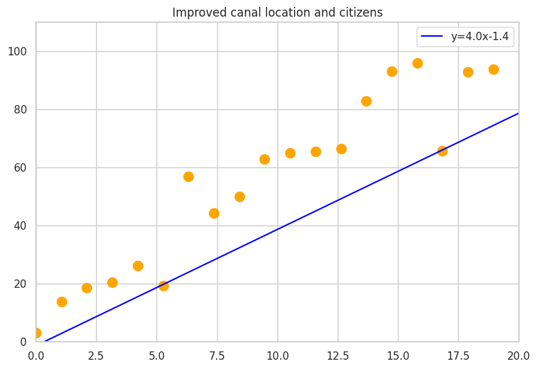
Improved canal location and citizens
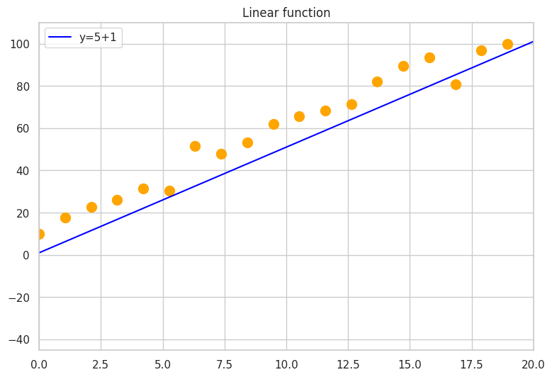
Now it’s better for most of the citizens. It’s the best solution for the village based on democracy, and the decision on where to dig the channel is found.
The best canal location
This is right river location if all votes are fair and the cost of each citizen
is a constant and equal to all other citizens.
Now let’s understand how we can find the best for any case river. And to do that SGD will help us.
Stochastic Gradient Descent (SGD)
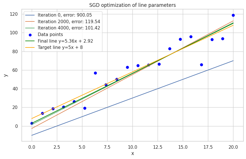
Now, we will discuss the algorithm for finding the best-fit line.
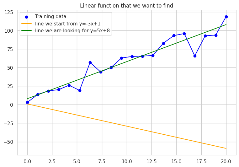
We have a training data set (x and y values). Our goal is to build the blue line
\( y_{\text{pred}} = a \cdot x + b \), which requires us to find the coefficients
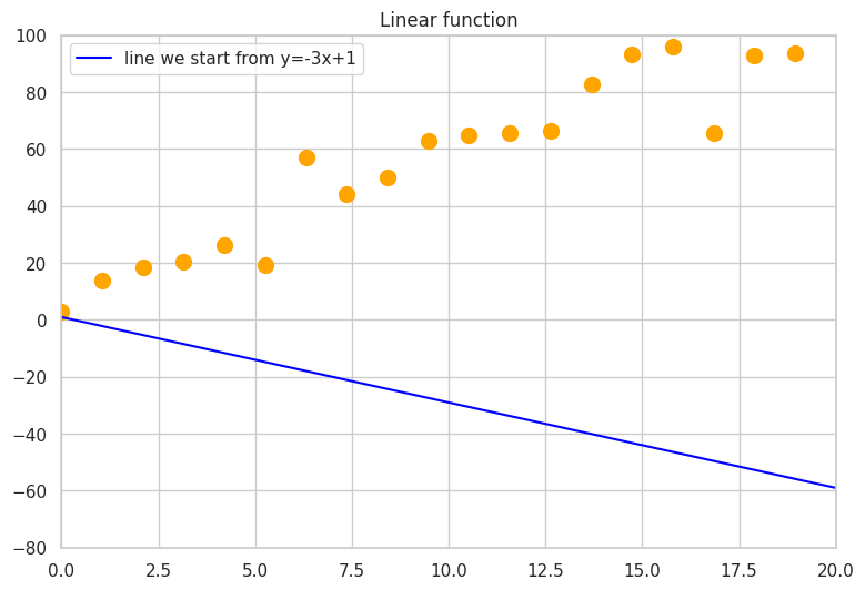
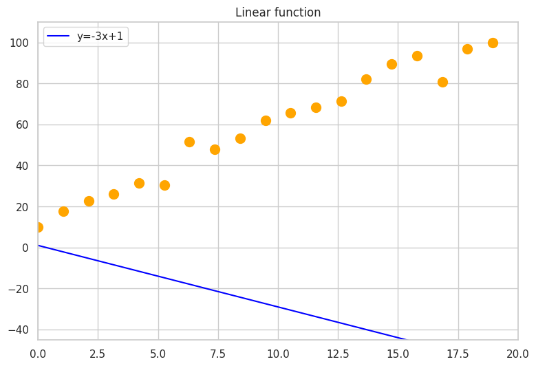
a and b. We initialize the values of a and b randomly; let them be
− 3 and 1 respectively for instance. The graphic below represents the line we
want to find, the points from the training data set, and the orange line we start
from in our search. The final line equation will be close to
\( y = 5 \cdot x + 8 \), but different, because we added some noise to the
y values, making the points not lie perfectly on one line, hence we will not be
able to get an error of 0.
Stochastic Gradient Descent. Each word in the title has a specific meaning.
"Descent" indicates that we want to minimize errors/distances to the lines,
and we need to change the line coefficients \(a\) and \(b\) in the opposite
direction to which the gradient indicates it grows. "Gradient" means we use
gradient information in the algorithm. "Stochastic" here means there’s a
probabilistic effect in the algorithm. In the simple realization below,
we won't use it. However, in more complicated examples, we usually don’t
train each iteration on the full dataset. It is done on a small piece of the
dataset for two reasons: easier calculation and random solutions help to find
different local/global minima.
We need to figure out correct a and b line parameters. We have MSE metric that we want to minimise,
gradients will help us to do that.
We have prediction. We want that prediction was as much closer to the right answer as possible. Than closer
a and b parameters to the ground true law, then smaller error.
\( y_{\text{pred}} = a \cdot x + b \)
The Mean Squared Error (MSE) is given by the formula
The most important part is that we need to have the partial derivatives of MSE for the
a and b parameters. Below is the general formula, but we have a training data set.
We calculate the gradient for each point by inserting x and the true values of y into the formula,
along with the current values of a and b. Then, we calculate the mean of these gradients,
as you will see in the code below. Afterward, we update a and b based on these gradients and the
learning rate (lr).
The learning rate determines the size of the updates toward improvements. It is important
because we can only trust the gradient locally, in a small area. If the learning rate is too small,
the learning process will be very slow as we will make very small updates. However, if the learning
rate is too large, we might step out of the local and global minimums and will not find the line with
the smallest error. Therefore, we need to find an optimal value for the learning rate.
The partial derivative of the MSE with respect to \( a \) and \( b \) are:
Prepare training data set (orange points (x, y)).
Initialize the line (parameters a and b) with random values.
Initialize lr (learning rate) to 0.001 - we make small steps in the direction opposite to the gradient.
Initialize number_of_iterations to 10000 (sufficient for this task).
Start loop:
1) Calculate predictions using line parameters a and b and the training data set x and y;
2) Calculate error to monitor that it decreases and ensure the algorithm works properly;
3) Calculate partial derivatives of a and b for MSE for all training points and find the mean
4) Update a and b slightly in the direction opposite to the gradient;
5) Repeat loop until any stop condition is met:
* Number of iterations is achieved;
* Error stops decreasing;
* All gradients are 0.
importnumpyasnpimportmatplotlib.pyplotaspltimportrandomfromrandomimportrandint# the line we will be searching forlinear=lambdax:5*x+8# good practice is to monitor error during optimizationdefmse(y_true,y_pred):returnsum((y_true-y_pred)**2)/len(y_true)if__name__=='__main__':random.seed(8)# lock seed to repeat experiment# creating training data set x and yx=np.array(range(20))y=np.array([linear(i)+randint(-10,10)foriinx])# initialize parameters of the line we will be optimizinga,b=random.randint(-10,10),random.randint(-10,10)# SGD part starts, initialize lr=0.0005# controls steps sizenum_iteration=10000# amount of time we want to update line# iterative process of searching for the line with the #smallest MSEforiinrange(num_iteration):pred=a*x+berror=mse(y,pred)# calculate partial derivativesdf_da=np.dot(x,2*(pred-y))/len(pred)df_db=sum(2*(pred-y))/len(pred)# update line parametersa-=lr*df_dab-=lr*df_dbifi%100==0:print(f"errors {error}")
Notice that you can delete 2 from derivative, because here it’s just multiplication to the constant what can be incorporated into learning rate.
So what we have
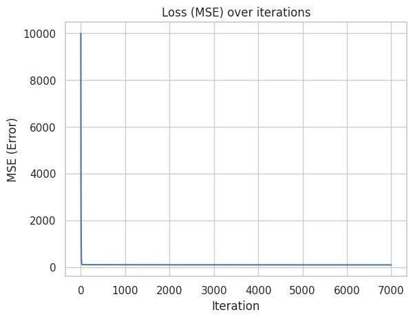
The main metric we have to monitor during training is error. If the error decreases everything goes right (in the most cases)
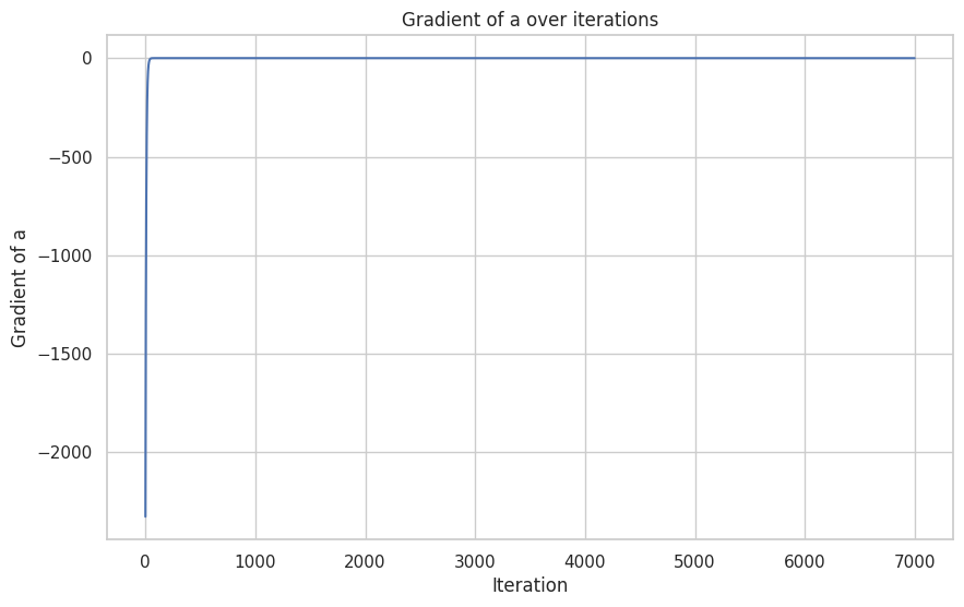
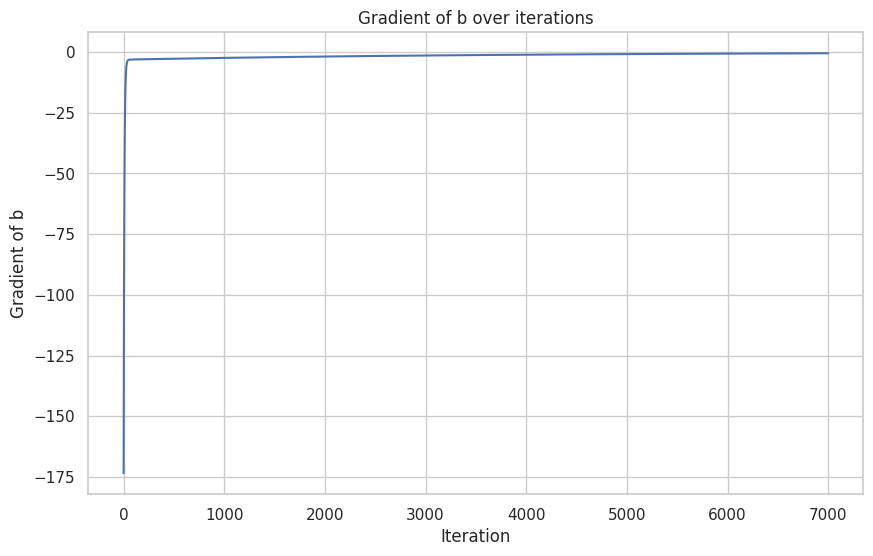
MSE loss, grad a and b for training process
You see that gradients were big in the beginning it changed parameters fast in the beginning because error was big - big-big gradients, than smaller error then smaller gradients to fix this error.
The second thing to note If you look at gradients of parameters a and b you can notice a few things.
You could stop iterations earlier d
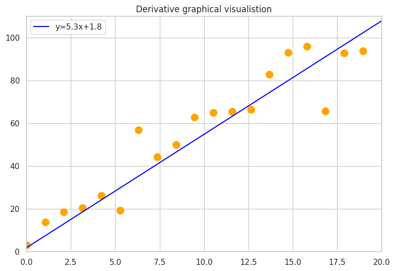
Line improvements during training
So, it was Linear Regression for general case.
Now in the end let's look at Some special cases.
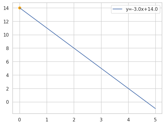
If we have one point in training data set, angle can be different and we have infinite number of solutions.
Case for one point, the right answers, different lines are possible
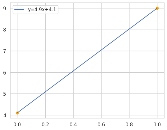
If we have 2 points we have only one solution, error is 0 and sum of square distances is 0.
Case for 2 points
For two dots the right answer is only 1 possible line, same as for all other amount of points.
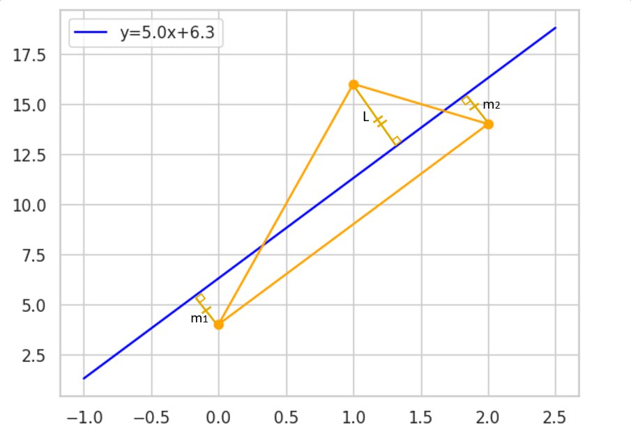
For three points, solution must be parallel to the longest side of triangle and L^2 must equal m12+m22.
3 Points
The smallest MSE is achieved when line is parallel the longest side and sum of squares distances from this
side is equal square of distance from the last third dot.
For four points more cases and so on.
Another thing to look at when we update only one out of two parameters only a or only b.
Line we start fromUpdate only b. We only change abscises value of the line, but not angle
Update only a. In that sense a is more important parameter to minimize the error which formulates the error.And a and b are updated. General case when everything is fine
Conclusion
We repeated how to build linear regression as well as other important for Deep
learning concepts as gradients and optimizers (SGD is the simplest one). The next
lesson will be devoted to Neuron Networks. We will try to solve spiral
classification network using Pytorch. Pytorch is popular autograd package for
deep learning in python. And the third important for understanding lesson-video
from Andrey karpathy how to build your own python autograd package same as
pytorch and also you will partially repeat what we have in the first two lesson.
This info is base which must be detailed learned and there’s no sense to move
forward to deep learning until you fully understand this consepts and materials.
See you on the second lesson!