Numpy
Here we look at some basic numpy functionality based on some statistical and theory probability examples.
NumPy is the package for scientific computing in Python. It is a Python library that provides a multidimensional array object, an assortment of routines for fast operations on arrays, including mathematical, logical, shape manipulation, sorting, selecting, I/O, discrete Fourier transforms, basic linear algebra, basic statistical operations, random simulation and much more.
At the core of the NumPy package, is the ndarray object. This encapsulates n-dimensional arrays of homogeneous data types, with many operations being performed in compiled code for performance. There are several important differences between NumPy arrays and the standard Python sequences:
1.From a Python List or Tuple:
import numpy as np

# From a list
array_from_list = np.array([1, 2, 3, 4, 5])

# From a tuple
array_from_tuple = np.array((1, 2, 3, 4, 5))
2.Creating Arrays with Default Values:
# Array of zeros
zeros_array = np.zeros((3, 4))  # 3x4 array of zeros

# Array of ones
ones_array = np.ones((2, 3))  # 2x3 array of ones

# Array with a constant value
full_array = np.full((2, 2), 7)  # 2x2 array filled with the value 7
3.Creating Arrays with a Range of Values:
# Array of evenly spaced values (step value)
range_array = np.arange(0, 10, 2)  # [0, 2, 4, 6, 8]

# Array of evenly spaced values (number of samples)
linspace_array = np.linspace(0, 1, 5)  # [0. , 0.25, 0.5 , 0.75, 1. ]
4.Creating Arrays with Random Values:
# Array with random values from a uniform distribution
random_array = np.random.random((2, 3))  # 2x3 array with random values

# Array with random integers
random_int_array = np.random.randint(0, 10, (3, 3))  # 3x3 array with random integers from 0 to 9
5.Creating Identity Matrix:
6.Creating Arrays with Specific Data Types:
# Array with a specified data type
int_array = np.array([1, 2, 3, 4], dtype=np.int32)  # Array of 32-bit integers
float_array = np.array([1.0, 2.0, 3.0], dtype=np.float64)  # Array of 64-bit floats
Each of these methods can be used based on what kind of array you need for your application. We will be using numpy in our work to generate and keep some data for training algorithms and RL agents. NumPy arrays are highly flexible and efficient for numerical operations in Python.
Statistics
Theory probability
In probability theory, the expected value (also called expectation, expectancy, expectation operator, mathematical expectation, mean, expectation value, or first moment) is a generalization of the weighted average. Informally, the expected value is the arithmetic mean of the possible values a random variable can take, weighted by the probability of those outcomes. Since it is obtained through arithmetic, the expected value sometimes may not even be included in the sample data set; it is not the value you would "expect" to get in reality.
The expected value of a random variable with a finite number of outcomes is a weighted average of all possible outcomes. In the case of a continuum of possible outcomes, the expectation is defined by integration. In the axiomatic foundation for probability provided by measure theory, the expectation is given by Lebesgue integration.
The expected value of a random variable X is often denoted by E(X) or E[X].
Small Spoiler
In the Reinforcement learning overall goal is to train such agent/policy that will maximize Expected value of total cumulative Reward which agent gets during interaction with Environment. Where xi will be calculated total discounted reward collected during trajectory t and pi is probability of that trajectory t.Discrete E(x):
Fair dice example
- outcomes: An array of possible outcomes for a 6-sided dice:
[1, 2, 3, 4, 5, 6]. - probabilities: Each outcome has a probability of \( \frac{1}{6} \) (for a fair dice).
- Expected Value: The expected value \( E(X) \) is calculated using the formula: $$ E(X) = \sum (x_i \cdot p_i) $$
where \( x_i \) is each outcome and \( p_i \) is the probability of that outcome.
The expected value for a fair 6-sided dice should be 3.5. Notice that Expected value must not be one of possible
outcomes of dice [1,2,3,4,5,6]. E(x)=3.5.
Show Python Code Examples
def expected_value_discrete(outcomes:list, probabilities:list):
    if len(outcomes) != len(probabilities):
        raise ValueError("Length of outcomes and probabilities lists must be the same.")

    expected_value = 0
    for i in range(len(outcomes)):
        expected_value += outcomes[i] * probabilities[i]

    return expected_value

outcomes = [1, 2, 3, 4, 5, 6]  # List of outcomes (e.g., dice values)
probabilities = [1 / 6, 1 / 6, 1 / 6, 1 / 6, 1 / 6, 1 / 6]  # List of corresponding probabilities expected_value =
expected_value_discrete(outcomes, probabilities)
Continuous E(x)
Instead of calculation definite integral using Newton-Leibniz formula we will see how we can calculate it programmatically with reals numbers
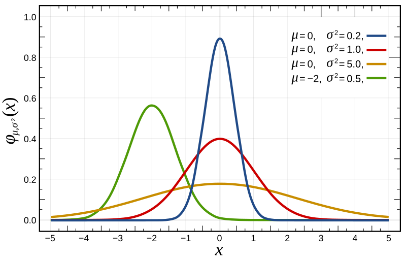
We have normal distribution with different mu and sigma presented below

Python code for Continuous E(x) for normal (Gaussian) distribution
def gaussian_pdf(x, mu, sigma,alpha):  # normal distribution
    return 1 / (sigma * math.sqrt(2 * math.pi)) * math.exp(-0.5 * ((x - mu) / sigma) ** 2)
def exponential_pdf(x, alpha):  # normal distribution
    if x<0:
      raise Exception("Exponential pdf is defined where x>0")
    return alpha*math.exp(-alpha*x)
def calculate_expected_value_continuous(pdf_function, lower_bound, upper_bound, mu=0, sigma=1, num_points=100000):
"""
Calculate the expected value for a continuous random variable and plots its graphic.
Parameters:
pdf_function (function): The probability density function of the random variable.
lower_bound (float): The lower bound of the integral.
upper_bound (float): The upper bound of the integral.
num_points (int): The number of points used in numerical integration (optional, default=10000).
Returns:
float: The expected value.
"""
step = (upper_bound - lower_bound) / num_points
x_values = [lower_bound + i * step for i in range(num_points + 1)]
probabilities = [pdf_function(x, mu, sigma) for x in x_values]
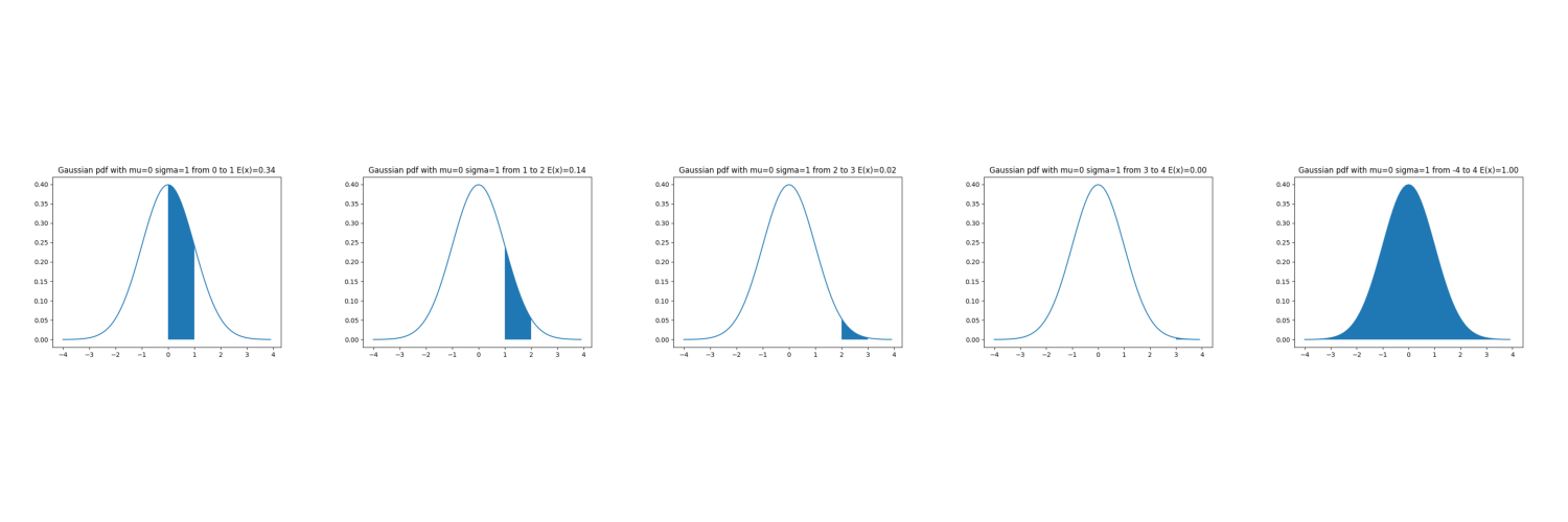
plt.plot(np.arange(-4, 4, 0.1), [pdf_function(x=i, mu=mu, sigma=sigma) for i in list(np.arange(-4, 4, 0.1))])
plt.fill_between(x_values, probabilities)
expected_value = 0
for i in range(num_points):
expected_value += step * probabilities[i]
plt.title(f"Gaussian pdf with mu={mu} sigma={sigma} from {lower_bound} to {upper_bound} E(x)={expected_value:.2f}")
plt.show()
return expected_value
if __name__ == '__main__':

    expected_value01 = expected_value_continuous(pdf_function=gaussian_pdf,
                                                 lower_bound=0,
                                                 upper_bound=1,
                                                 mu=0,
                                                 sigma=1)
    expected_value12 = expected_value_continuous(pdf_function=gaussian_pdf,
                                                 lower_bound=1,
                                                 upper_bound=2,
                                                 mu=0,
                                                 sigma=1)
    expected_value23 = expected_value_continuous(pdf_function=gaussian_pdf,
                                                 lower_bound=2,
                                                 upper_bound=3,
                                                 mu=0,
                                                 sigma=1)
    expected_value34 = expected_value_continuous(pdf_function=gaussian_pdf,
                                                 lower_bound=3,
                                                 upper_bound=4,
                                                 mu=0,
                                                 sigma=1)
    expected_value44 = expected_value_continuous(pdf_function=gaussian_pdf,
                                                           lower_bound=-4,
                                                           upper_bound=4,
                                                           mu=0,
                                                           sigma=1)
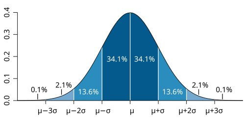
print("Chance (probability) that element sampled from normal distribution with mu=0, sigma=1 lies in diapason of:")
print(f"\t one variance {2*expected_value01*100:.2f}%")
print(f"\t two variance {2*(expected_value01+expected_value12)*100:.2f}%")
print(f"\t three variance {2*(expected_value01+expected_value12+expected_value23)*100:.2f}%")
print(f"\t four variance {2*(expected_value01+expected_value12+expected_value23+expected_value34)*100:.2f}%")

print(f"Let's check ourself: {expected_value44*100:.2f} What is correct!")

General case and above we had an example with concrete values.

All kinds of variables in natural and social sciences are normally or approximately normally distributed. Height, birth weight, reading ability, job satisfaction or SAT scores are just a few examples of such variables.
Ok there's a task A light bulb is given. The likelihood that it will burn out during some period of time does not depend on how long it has already worked, but depends only on the duration of the period of time. The probability that the light bulb will last from 2000 to 6000 hours is 37.5%; What is the probability that a light bulb will last less than 2000 hours?
Let \( T \) be the lifetime of the lightbulb, modeled as an exponential distribution. The cumulative distribution function is:
Given that \( P(2000 < T \leq 6000) = 37.5\% \), we set up the equation:
Substitute the exponential formula:
Let \( x = e^{-\lambda \cdot 2000} \), then:
Solving for \( x \), we then calculate \( \lambda \) using \( x = e^{-\lambda \cdot 2000} \).
Finally, the probability that the lightbulb lasts less than 2000 hours is:
You could use defined integral, or find lambda but we used variable exchange trick to solve this task So probability that light bulb will be burned out before 2000 hours usage is 50% and decreases with time with exponential distribution. So different types of distributions can be useful, for example other types of distributions are used to initialize some weights of neuron networks that gives or helps to achieve different neuron network properties to help or improve the training process.
Task 1. Modify the code above a bit to solve this task numerically. You should change pdf function to exponential and insert correct lambda value.